Class conditional and class generic disentangled representations

During my internship at IIT-H, I came across disentangled representations while going through the ICML paper Disentangling by factorising. In this work by Kim et al, Factor-VAE, modeling of the disentangled representations is done by encouraging the marginal distribution of representation to be factorial. They achieved this by minimizing the total correlation(TC) of the latent units- where we define the TC of a set of random variables \(z_1,z_2,...z_n\) as \begin{equation} TC(z_1,z_2,…,z_n)= KL(p(z_1,z_2,…,z_n)||\prod_{i=1}^{n}p(z_i)) \end{equation} (Here \(KL\) stands for Kullback-leibler divergence). They estimated TC by using density ratio estimation.

Problem

Factor-VAE learns a generalised set of factors of variation for all the classes in a dataset,i.e, using Factor-VAE, we can model only those factors which are common to all the classes. But, what if we want to learn class specific factors? or if we want to understand the class-specific properties? using Factor-VAE, we are forced to learn as many models as there are classes which is quite cumbersome, thus, it’s not desirable. In order to address this problem, we proposed a solution.

Assumptions and approach

We assume that we have a dataset \(\mathbb{D}\) of samples \((x,y)\) with \(n\) classes where \(x\) is our observation and \(y\) is it’s one-hot encoded class label belonging to\(\{y \in \{0,1\}^{n} \mid \sum_i(y_i)=1\}\). We consider a VAE kind of setup for our experiments and problem solving. Since we are interested in learning disentangled representations which take the class information into consideration, the obvious choice is to explicitly condition the encoder with the class label for learning representations with cues from the class label.

naive-model

We consider the set of latent variables to be denoted by \(\textbf{z}\) and we define a posterior \(q_{\phi}(z|x,y)\), a prior \(p(z|y)\) and likelihood \(p_{\theta}(x|z,y)\) This model’s framework is similar to a fully supervised conditional VAE setup, where we try to optimize the variational lower bound \begin{equation} p(x|y) \geq E_{q_{\theta}(z|x,y)}[p(x|z,y)] - KL(q_{\theta}(z|x,y)||p(z))
\end{equation} But in our case since we want to learn disentangled representations, like in \(\beta-\)VAE, we have an additional weight on the KL-divergence term to ensure disentanglement of the variables. The problem with this objective is quite clear, similar to that of \(\beta-\)VAE’s the additional weight that we put on KL-divergence term is adding on to minimizing the mutual information between \(z\) and the joint variable \((x,y)\) w.r.t the variational joint distribution as well. Hence, even though the \(z\) gets disentangled, the latent code’s knowledge about the data is minimized in every step. This can be easily shown following the Makhzani et al and proof in Factor-VAE. \begin{align} E_{(x,y)\sim D(x,y)}[KL(q_{\theta}(z|x,y)||p(z))] = I(z;(x,y))+KL(q(z)||p(z)) \end{align} We generally take standard gaussian as \(p(z)\), so the representation \(q(z)\) gets disentangled because of the weight term. To restrict the problem aroused by \(I(z;(x,y))\), we can put a cap on the \(KL\) term in this objective with a gradually increasing positive term \(C_z\) and modify our objective similar to that of burgess et al’s. Using an approach like this simply narrows down our intent for learning meaningful representations. We expect to learn factors both which are and which are not affected by class-information. To solve this problem, we can use the following model, the details of which are explained in the next subsection.

Proposed Model

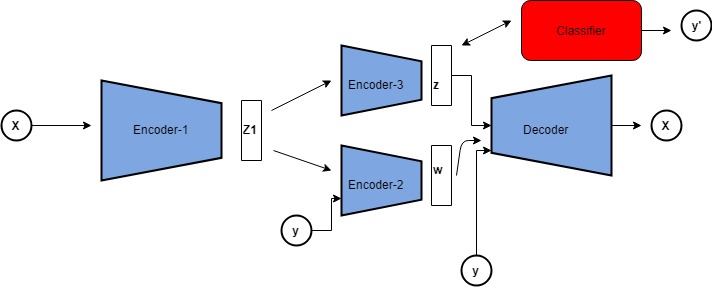
We propose a model which is a modification to the previous model’s framework which allows us to model both class-dependent and class-independent factors. Let \(\textbf{z}\),\(\textbf{w}\) denote the set of class-dependent and class-independent variables respectively. We define a joint posterior \(q_{\phi}(z,w|x,y)\), a prior \(p(z,w|y)\) and likelihood \(p_{\theta}(x|z,w,y)\). With this premise, the conventional \(\beta\)-VAE kind of objective is, \begin{equation} L(\theta,\phi)= E_{q_{\phi}(z,w|x,y)}[p_{\theta}(x|z,w,y)]-\beta .KL(q_{\phi}(z,w|x,y)||p(z,w|y)) \end{equation} Since we have assumed that \(z \perp y\) and \(z \perp w\), we rewrite this objective as \begin{equation} L(\theta,\phi)= E_{q_{\phi}(z,w|x,y)}[p_{\theta}(x|z,w,y)]-\beta .KL(q_{\phi}(z|x)||p(z|y)) - \gamma .KL(q_{\phi}(w|x,y)||p(w|y)) \end{equation} Taking inspiration from burgess et al, we put a cap on the KL-divergence terms so that there is not much information about the data lost. With this our modified objective is \begin{align} L_{VAE}= E_{q_{\phi}(z,w|x,y)}[p_{\theta}(x|z,w,y)]-\beta|KL(q_{\phi}(z|x)||p(z|y)) - C_z| - \gamma|KL(q_{\phi}(w|x,y)||p(w|y)) - C_w| \end{align}

Minimizing class dependence

We have assumed that \(z \perp y\) and we wanted most information related to \(y\) to dwell in \(w\), so we explicitly minimize the mutual information between \(z\) and \(y\). We do this by making use of a classifier network. If \(z \perp y\), the classifier misclassifies a given \(z\). For this purpose, we define an augmented loss to be maximized by the network using a binary-cross-entropy. \begin{align} & L_{class}(z)= y.log(\sigma(h_{\psi}(z))) + (1-y).log(1-\sigma(h_{\psi}(z))) \end{align} Since the classifier must also be capable of predicting the correct class label given \(z\), the classifier’s parameters are also to be trained to achieve the below defined objective- \begin{alignat}{2} \min_{\psi} \quad && L_{class} \end{alignat} So, our overall objective is to solve the below multi-step optimization problem where we train the parameters of encoder and decoder by solving the maximization problem in the first-step and train the parameters of the classifier in the next step while solving the minimization problem- \begin{align} & \max_{\theta,\phi} \quad && L(\theta,\phi)+ L_{class} \end{align} \begin{align} & \min_{\psi} \quad && L_{class} \end{align}

Results and experiments

I tested this model on 3 datasets: MNIST, Fashion-MNIST, CelebA. I noticed some pretty good results on MNIST and FMNIST where I was able to generate multiple class-dependent features.

Qualitative results

Class-specific factors(W|y)

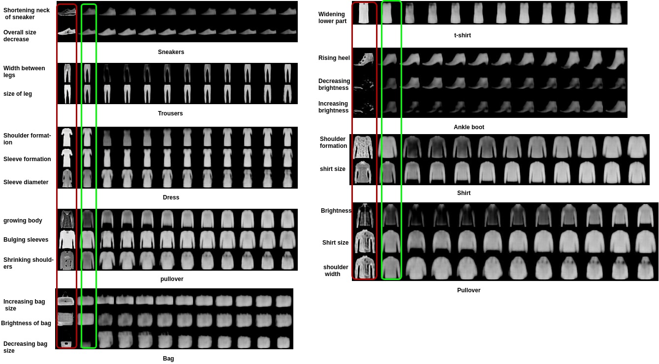
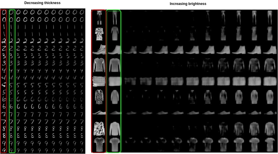
I have clearly pointed out factors we identified for each class. We can understand what each factor corresponds to by traversing between -5 and 5 along a particular dimension of the latent \(w\) and by keeping the values across all other dimesnions to be constant. The reconstructions along each row correspond to the samething done(Images in Red correspond to original images and the ones in green are their reconstructions). The qualitative results are shown below: The above image depicts the various class-specific factors that are observed in Fashion-MNIST dataset. The above image depicts the various class-specific factors that are observed in MNIST dataset.

Generic factors of variation(Z)

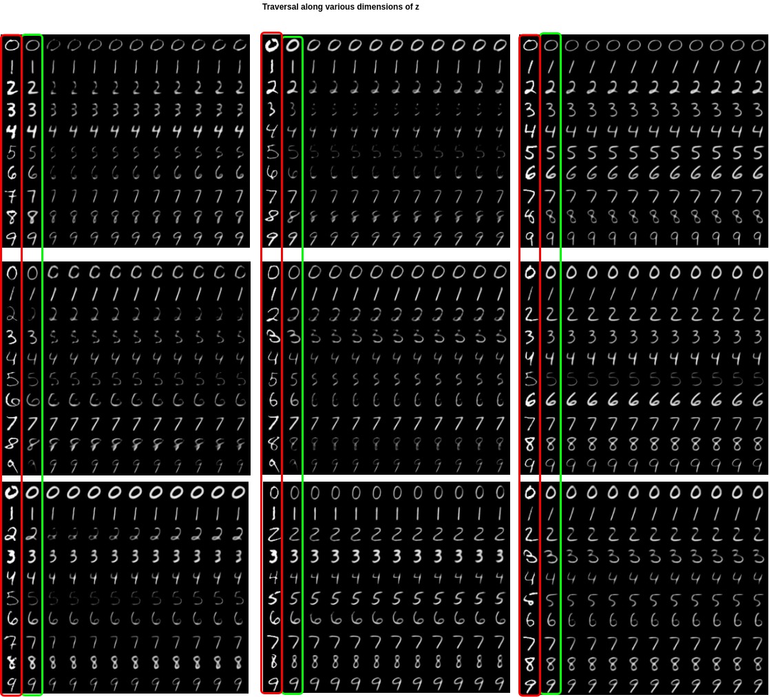
The below results depict the factor that was learnt by the model. Each row corresponds to reconstructions observed while varying one particular dimension of the latent representation \(z\) between -5 and 5. We noticed that, for a particular dimension, same factor can be seen to be varying for all the classes which is what was intended. Above image corresponds to the factor that is common to all the classes in that dataset.

Each block corresponds to reconstructions observed while varying one particular dimension of the latent representation \(z\) between -5 and 5. We noticed that, for that particular dimension, either no common factor or some meaningless variation can be seen to be varying for all the classes which is what was intended.

Quantitative results

To check the extent to which our objective has helped in channeling the class-information from \(z\) to \(w\), we have trained separate classifiers(with same capacity) on samples from \(z\) and \(w|y\) respectively to predict their respective class labels with and without using \(L_{class}\) on the datasets MNIST,Fashion-MNIST and CelebA. The accuracies we are mentioning here are the average accuracies of \(3\) runs. We took this average to avoid misjudgment caused due to randomization. It can be clearly observed that in all the \(3\) datasets that we have tested upon, the case when using \(L_{class}\) is helping \(w\) in achieving higher accuracy in predicting the true label. This gives enough validation to our intent for the class-specific information to reside in \(w\) and non-class specific information to be in \(z\).

Dataset	Method	Accuracy on z	Accuracy on w
Fmnist	without L-class	0.337	0.47
Fmnist	with L-class	0.32	0.68
Mnist	without L-class	0.37	0.31
Mnist	with L-class	0.30	0.45
CelebA	without L-class	0.63	0.68
CelebA	with L-class	0.685	0.745

Written on October 1, 2019