Nearest Neighbor classifier
This post is about(probably) one of the most simple algorithms of ML- Nearest Neighbor classifier. To begin with, it’s a known fact that the whole concept of ML relies on a crucial idea called the “plug-in principle”. This blog is a nice read for the people interested in learning the basics of statistical foundations of ML. Nearest Neighbor algorithm is one of the many algorithms that branched out of this principle.
Problem setup
we are given a training set \(S = \{(X_1, Y_1), (X_2, Y_2),......, (X_n, Y_n)\}\) and a testset \(T = \{X_1', X_2',......, X_m'\}\), we’re supposed to train/ develop/ learn a model using the points in \(S\) and predict the corresponding \(Y_i \forall X_i \in T\). Here \(X_i \in \mathbb{R}^d\) and \(Y_i \in \{0,1,2,...,8,9\}\).
Assumption in Nearest Neighbor classifier
This algorithm assumes that are the \(X_i \in S\) having identical \(Y_is\) exist in a cluster, i.e., any point in the dataset has the label equivalent to the label possessed by the point ‘closest’ to it. There are many metrics to assess this ‘closeness’.
Further setup for this post
The most commonly used metric is the \(\ell_2-norm\)(Of course, it doesn’t make sense to use this metric for every problem). This makes sense in this setup because we have already defined that our inputs belong to the Euclidean space. This post will be primarily focused on simplifying/ optimizing the implementation of nn-classifier when using the Euclidean distance metric. This optimization is based on a mathematical trick.
Details
So, if we want to assign label to every point in the test data, we need to find the \(\ell{}_2-distance\) between every vector/input and every vector/ point in the test data. Oh yeah, this seems like quite cumbursome, but yes, it’s certainly inevitable(like Thanos!). If you want to do the below operation, I’m telling you it’s going to take a lot of time.
for x_j,y_j in S:
    for t_i in T:
        distance = np.square(x_j-t_i).sum()
Instead, let’s skip the part using 2 for loops- as numpy has some cool array-operations that can optimize our implementation. We should use the below identity for finding the euclidean distance between two vectors \(x_j, t_i\): \begin{equation} ||t_i - x_j||^2_2 = (t_i - x_j)^T(t_i - x_j) = t_i^Tt_i + x_j^Tx_j -2t_i^Tx_j \end{equation} For the last term we need to compute the product of the matrices(as we’re dealing with matrices in our implementation not individual vectors). We can’t escape doing the product of the two big arrays \(X, T\) for the last term, so instead I focused on optimizing the way we find the first two terms:
Optmization -1
If we observe carefully, the first and second terms: \(t_i^Tt_i, x_j^Tx_j\) involve taking the dot product of the vectors with themselves. So we can simply take the product \(S^T.dot(S)\) and \(T^T.dot(T)\), and pick the diagonal elements from the obtained matrices.
    t_square = (test.dot(test.transpose())).diagonal()
    x_square = (X.dot(X.transpose())).diagonal()
We can see that this still involves multiplying big matrices, below is the further optimization.
Optimization -2
If we notice carefully, the first two terms represent square of lengths of every vector as \(x_j^Tx_j=||x_j||_2^2\). We can simply square the indivdual elements in \(S, T\) and sum along the axis=1. This will also give the lengths of vectors as in the earlier results.
    t_square = np.square(test).sum(-1)
    x_square = np.square(X).sum(-1)
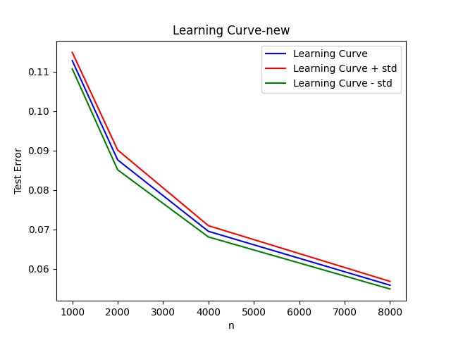
To test the efficacy of these steps, I did a simple experiment: I picked the MNIST dataset, For each \(n \in \{1000, 2000, 4000, 8000\}\):
- Draw n points from data, together with their corresponding labels, uniformly at random.
- Use these n points as the training data and testdata as the test points; compute the fraction
of test examples on which the nearest neighbor classifier predicts the label incorrectly (i.e.,
the test error rate)
This is the plot of the learning curve when using the nearest neighbor algorithm
 I carried out the above two steps 10 times for every \(n\).
The first optimization step took 222.86 seconds, and the second optimization took 111.9936. That means, a simple understanding of what norm is, has reduced our runtime by alomst half. I have uploaded these two implementations on my github account- Optimization-1, Optimization-2. Please keep checking this blog for further cool posts.
